Ribo-seq pipeline steps and reports
Analysis pipeline steps
Initial steps are similar to described in Ingolia et al. Nature 2012
Filtering Sequences:
- Cutadapt:
Keep sequences 20-50 bp that have an adapter. Remove adapter and the first base.
Align to rRNA Transcripts:
- Bowtie:
Align sequences to rRNA transcripts. Keep sequences that do not align.
Filtering for Reads of Length 28-33:
- Cutadapt:
Filter reads to keep sequences of length 28-33 bp.
Align to Genome:
- Tophat:
Align the filtered sequences to the genome.
Create Coverage Files:
- IGVTools:
Create TDF files for coverage visualization.
Quantify 5’UTR and CDS:
- HTSeq:
Quantify 5’UTR and CDS regions.
Discover Ribosomal Profiling Summits:
- MACS:
Identify ribosomal profiling summits.
- IntersectBed & awk:
Shift and expand summits. Annotate the summits.
Summarized points:
Sequence data: Including file format conversion and/or demultiplexing
Filter sequences: keep sequences that have adapter and that after adapter remivl are atleast 20 bases long
2a. Run QC
Align to rRNA transcripts and filter sequences that align
Filter sequences to keep sequences between footprint length 24-35
5a. Run QC
Align cDNA to genome
6a. Make coverage files (tdf)
6b. Calculate coverage on 5’UTR and CDS
Find peaks summits
Extend and annotate summits

Pipeline report
Upon completion of the analysis, you will be sent an email with links to the results report.
The report includes several sections:
Sequencing and Mapping QC
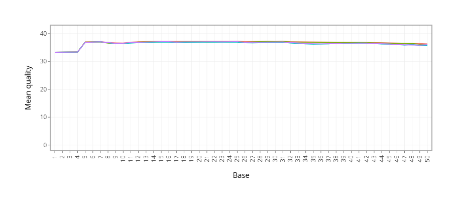
Figure 1 - Plots the average quality of each base across all reads. Qualities of 30 (predicted error rate 1:1000) and above are good.
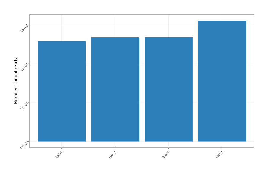
Figure 2 - Histogram showing the number of reads for each sample in the raw data.
Figure 3 - Histogram showing the percentage of reads discarded after trimming the adapters (after removing adapters, short, polyA/T and low quality reads are discarded by the pipeline). No figure will be presented if the percentage of reads discarded after trimming for all samples is lower than 1%.
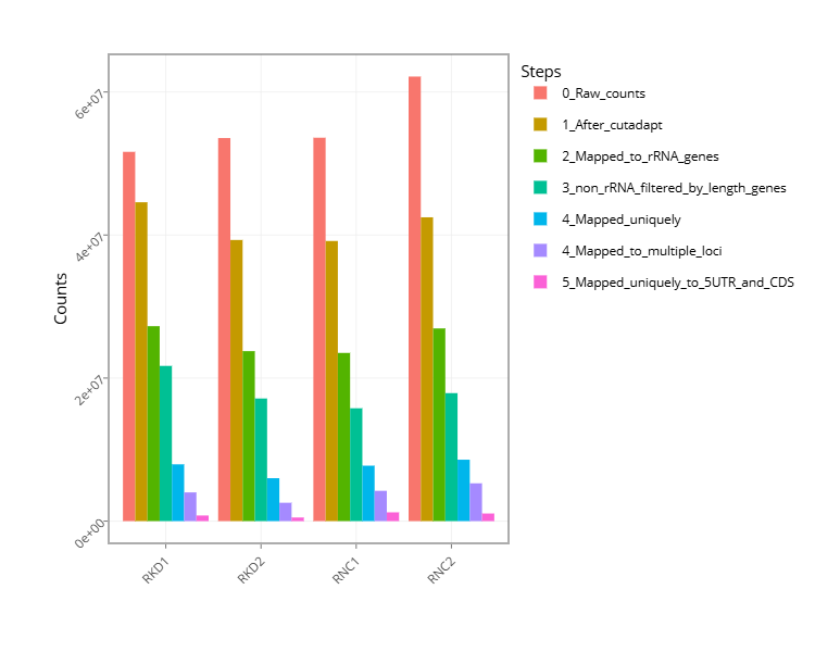
Figure 4 - Histogram with the number of reads for each sample in each step of the pipeline.
- MACS peak calling
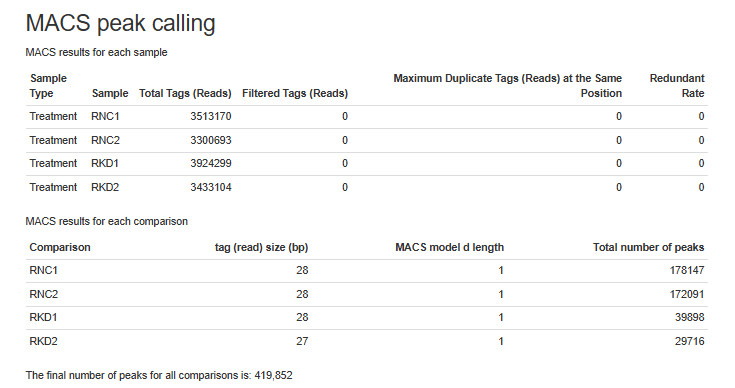
Figure 5 - MACS (peak calling) results table for each sample.
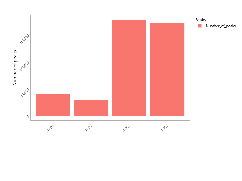
Figure 6 - Histogram with the number of peaks for all samples.
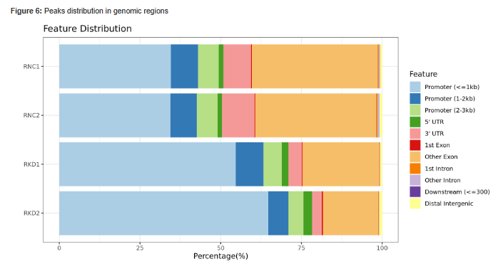
Figure 7 - Histogram showing Peaks distribution in genomic regions.
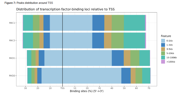
Figure 8 - Histogram showing Peaks distribution around TSS.
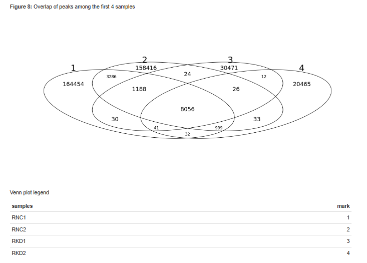
Figure 9 - Venn diagram of peak overlaps among the first four comparisons.
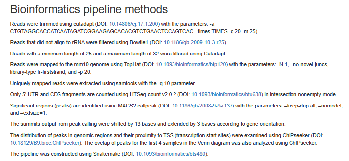
Bioinformatics Pipeline Methods - Description of pipeline methods.
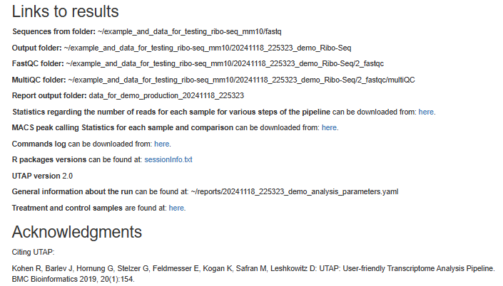
Links to additional results - Links for downloading tables with raw, normalized counts, log normalized values (rld), and statistical data of contrasts.
Output folders
1_cutadapt
2_fastqc
3_bowtie_rRNA
4_cutadapt_filter_length
5_fastqc
6_multiQC
7_tophat
8_samtools_filter
9_tdf
10_count_reads
11_merge_htseq_counts
12_macs_peaks
13_shif_and_extend_summit
14_reports
Log directory
Annotation file
For Peak annotation, we use annotation files (gtf format) from “Ensembl” or “GENCODE”.